Tutorial - Genomic annotation
This tutorial demonstrates the usage of gat with a simple example - where does a transcription factor bind in the genome?
As opposed to Tutorial - Interval overlap we will not be looking at the overlap between one set of intervals with another, but at the overlap of one set of intervals with multiple others.
This tutorial uses the SRF data set described in Valouev et al. (2008). The data sets used in this tutorial are available at:
http://www.cgat.org/~andreas/documentation/gat-examples/TutorialGenomicAnnotation.tar.gz
The data is in srf.hg19.bed.gz. This bed formatted file
contains 556 high confidence peaks from the analysis of Valouev et al. (2008)
mapped to human chromosome hg19.
We build the analysis in multiple steps. First, we will perform a simple analysis, which will also motivate the use of gat. Later, we will build more sophisticated analyses that take into account the effective genome.
First analysis
gat requires three sets of intervals:
- a set of segments delineating the active part of the genome (workspace), and
- a set of segments of interest (tracks), and
- a set of segments with annotations.
gat accepts bed formatted files as input.
As segments of interest we will be using the srf.hgf19.bed.gz
containing the results of the ChIP-Seq experiment:
chr5    60627981        60628031        SRF.1
chr5    137801055       137801105       SRF.2
chr5    137800766       137800816       SRF.3
chr7    5570273 5570323 SRF.4
chr5    137827838       137827888       SRF.5
...
As our workspace we will for now use the bed formatted
contigs.bed, which simply lists all chromosomes in hg19:
chr13   0       115169878       ws
chr12   0       133851895       ws
chr11   0       135006516       ws
chr10   0       135534747       ws
chr17   0       81195210        ws
...
As our annotations file, we will use the
annotations_geneset.bed.gz.
This file required a little more effort to build. We took all protein genes of Ensembl (release 67) and merged the exons of all transcripts of a gene. Based on these gene definitions we then divided genomic regions into intergenic, intronic and exonic regions. We also annotated the UTR (5’ and 3’), and the 5kb flank upstream and downstream. The result is a set of non-overlapping intervals covering the full genome:
...
chr1    362640  367639  5flank
chr1    367640  367658  UTR5
chr1    367659  368594  CDS
chr1    368595  368634  UTR3
chr1    368635  373634  3flank
chr1    373635  616058  intergenic
chr1    616059  621058  3flank
chr1    621059  621098  UTR3
chr1    621099  622034  CDS
chr1    622035  622053  UTR5
chr1    622054  627053  5flank
...
We can now run gat by giving specifying the three input files:
gat-run.py --ignore-segment-tracks --segments=srf.hg19.bed.gz
   --annotations=annotations_geneset.bed.gz --workspace=contigs.bed.gz
--num-samples=1000 --log=gat.log > gat.out
The option –ignore-segment-tracks tells gat to ignore the fourth column in the tracks file and assume that all intervals in this file belong to the same track. If not given, each interval would be treated separately.
The above statement finishes in a few seconds. With large interval collections or many annotations, gat might take a while. It is thus good practice to always save the output in a file. The option –log tells gat to save information or warning messages into a separate log file.
The first 11 columns of the output file are the most informative:
| track | annotation | observed | expected | Ci95low | CI95high | stddev | fold | l2fold | pvalue | qvalue |
|---|---|---|---|---|---|---|---|---|---|---|
| merged | intergenic | 5800 | 14056.3300 | 13100.0000 | 15000.0000 | 583.7181 | 0.4126 | -1.2771 | 1.0000e-03 | 1.5714e-03 |
| merged | intronic | 8816 | 10633.8530 | 9665.0000 | 11602.0000 | 592.7589 | 0.8291 | -0.2705 | 1.0000e-03 | 1.5714e-03 |
| merged | UTR3 | 233 | 278.0720 | 100.0000 | 493.0000 | 117.3112 | 0.8379 | -0.2551 | 3.6500e-01 | 4.4611e-01 |
| merged | 3flank | 800 | 659.6560 | 400.0000 | 1000.0000 | 175.0544 | 1.2128 | 0.2783 | 2.3100e-01 | 3.1762e-01 |
| merged | CDS | 754 | 360.7680 | 161.0000 | 580.0000 | 127.2204 | 2.0900 | 1.0635 | 1.0000e-03 | 1.5714e-03 |
| merged | flank | 1334 | 167.8620 | 50.0000 | 350.0000 | 91.4581 | 7.9470 | 2.9904 | 1.0000e-03 | 1.5714e-03 |
| merged | 5flank | 6524 | 691.5400 | 400.0000 | 1000.0000 | 185.0053 | 9.4340 | 3.2379 | 1.0000e-03 | 1.5714e-03 |
| merged | UTR5 | 3441 | 87.0110 | 0.0000 | 200.0000 | 60.9119 | 39.5467 | 5.3055 | 1.0000e-03 | 1.5714e-03 |
The first two columns contain the name of the track and annotation that are being compared. The columns observed and expected give the observed and expected nucleotide overlap, respectively, between the track and annotation.
The following columns CI95low, CI95high, stddev give 95% confidence intervals and the standard deviation of the sample distribution, respectively.
The fold column is the fold enrichment or depletion and is computed as the ratio of observed over expected. The column l2fold is the log2 of this ratio.
The column pvalue gives the empirical p-value, i.e. in what proportion of samples was a higher enrichment or lower depletion found than the one that was observed.
The column qvalue lists a multiple testing corrected p-value. Setting a qvalue threshold and accepting only those comparisons with a qvalue below that threshold corresponds to controlling the false discovery rate at that particular level.
What does this table tell us? Looking at the column observed only, we see that most binding of SRF occurs in intronic and intergenic regions:
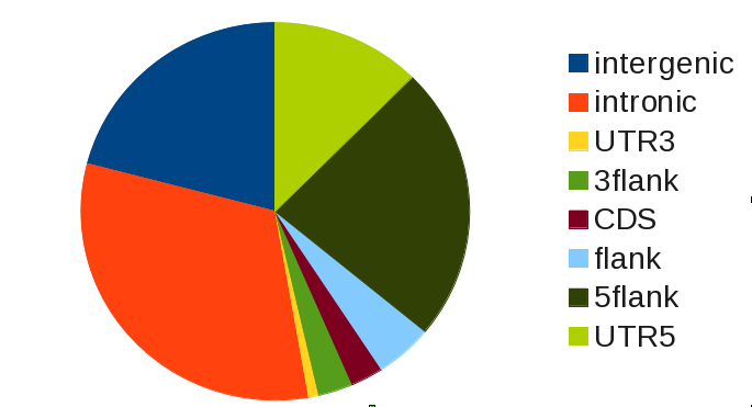
Strictly speaking, this is a a naive analysis that does not require gat. The observed overlap alone does not tell us if the overlap we see is more or less than we expect. We do know that there are much more and larger intronic regions than there are UTRs, for example.
More instructive is to look at the enrichment within the various genomic regions, which is given by the fold change.
Here, we clearly see that SRF binds preferentially at transcription start sites (UTR5 and 5flank), while its binding is actually less than expected in introns and intergenic regions.
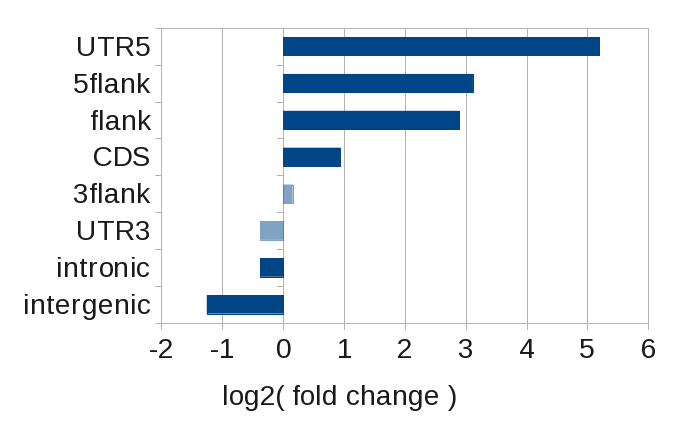
Binding distribution of SRF with respect to known protein coding genes. Plotted is the log2(fold change). Value not significant are transparent.
The effective genome
In the previous analysis we used the complete genome (3.1Gb) as the workspace. However, that is not realistic. For example, SRF will not be predicted in regions that are assembly gaps. Generally speaking, if the workspace is too large, fold enrichment values will be too optimistic.
To get a more accurate estimate of the enrichment in various regions, we should exclude assembly gaps.
The bed formatted file contigs_ungapped.bed.gz contains
only those genomic regions that are not assembly gaps (2.86Gb).
We can use this file instead:
gat-run.py --ignore-segment-tracks --segments=srf.hg19.bed.gz
   --annotations=annotations_geneset.bed.gz --workspace=contigs_ungapped.bed.gz
   --num-samples=1000 --log=gat.log > gat.out
| annotation | observed | expected | fold | l2fold | pvalue | qvalue |
|---|---|---|---|---|---|---|
| intergenic | 5800 | 13806.4540 | 0.4201 | -1.2512 | 1.0000e-03 | 2.2000e-03 |
| UTR3 | 233 | 303.6340 | 0.7674 | -0.3820 | 2.5300e-01 | 3.9757e-01 |
| intronic | 8816 | 11473.2200 | 0.7684 | -0.3801 | 1.0000e-03 | 2.2000e-03 |
| 3flank | 800 | 713.4290 | 1.1213 | 0.1652 | 3.4000e-01 | 4.6750e-01 |
| CDS | 754 | 391.1840 | 1.9275 | 0.9467 | 5.0000e-03 | 9.1667e-03 |
| flank | 1334 | 182.0200 | 7.3289 | 2.8736 | 1.0000e-03 | 2.2000e-03 |
| 5flank | 6524 | 761.1600 | 8.5711 | 3.0995 | 1.0000e-03 | 2.2000e-03 |
| UTR5 | 3441 | 97.3670 | 35.3405 | 5.1433 | 1.0000e-03 | 2.2000e-03 |
The associated fold changes change, albeit not much. But have we done enough? The SRF intervals are the result of a ChIP-Seq experiment. Because these were short reads (25bp), not all can be unambiguously mapped to a unique genomic location. This again effectively removes some genomic regions from the analysis.
The bed formatted mapability_36.filtered.bed.gz
contains all those genomic regions, that are uniquely mapable with
reads of 24 bases. These regions have been derived from the UCSC
mapability tracks and reduce the effective genome considerably
(1.96Gb).
We could intersect the two bed files ourselves, but we can also supply multiple workspaces to gat. gat will automatically intersect multiple workspaces:
gat-run.py --ignore-segment-tracks --segments=srf.hg19.bed.gz
   --annotations=annotations_geneset.bed.gz
   --workspace=contigs_ungapped.bed.gz
   --workspace=mapability_36.filtered.bed.gz
   --num-samples=1000 --log=gat.log > gat.out
As a consequence of reducing the workspace the fold changes change:
| annotation | observed | expected | fold | l2fold | pvalue | qvalue |
|---|---|---|---|---|---|---|
| intergenic | 5800 | 12531.2490 | 0.4628 | -1.1114 | 1.0000e-03 | 1.6000e-03 |
| UTR3 | 233 | 385.1620 | 0.6049 | -0.7251 | 1.1000e-01 | 1.2571e-01 |
| intronic | 8816 | 10942.7440 | 0.8056 | -0.3118 | 1.0000e-03 | 1.6000e-03 |
| 3flank | 800 | 625.3780 | 1.2792 | 0.3553 | 1.6500e-01 | 1.6500e-01 |
| CDS | 754 | 540.3700 | 1.3953 | 0.4806 | 8.2000e-02 | 1.0933e-01 |
| flank | 1334 | 166.6400 | 8.0053 | 3.0010 | 1.0000e-03 | 1.6000e-03 |
| 5flank | 6524 | 638.2110 | 10.2223 | 3.3537 | 1.0000e-03 | 1.6000e-03 |
| UTR5 | 3441 | 122.2010 | 28.1585 | 4.8155 | 1.0000e-03 | 1.6000e-03 |