Interpreting GAT results

Fold change

Gat reports fold changes. Fold change is simply expressed as a ratio of an observed metric compared to the expected value of the metric based on randomizations.

Fold changes of a single set of segments of interest against various annotations can be compared directly. Indeed, the primary objective of randomization is to remove the differences between number and segment sizes of different annotations in order to make them comparable. For example, the fold change of a set of transcription factor sites in promotors can directly be contrasted with the fold change of the same sites in introns.

When comparing the fold enrichment of multiple sets of segments of interest against the same annotation, some caution must be exercised. Here, the question is to compare the fold change of sites of transcription factor A in promotors with the fold change of sites of transcription factor B in promotors.

The difference becomes apparent when there is no observed overlap between the segments of interest and the annotations to be compared. In order to avoid division by 0, gat adds a pseudocount of 1 to observed and expected values: fc = (observed + 1) / (expected + 1). With no observed overlap, this becomes fc = (1 / expected + 1 ). The amount of expected overlap correlates with the number and size of segments in the segments of interest. If there are more sites for A than for B, the expectation of overlap is larger for A than for B. Thus, even if there is no overlap in both cases, the fold change values reported will be different. In the case of multiple annotations of different sizes, the annotations with no overlap for both A and B will lie along a straight line.

There is no such bias if there is overlap between the segments of interest and the annotations. As both the observed and the expected overlap depend upon the segment size and number of segments of the segments of interest, the effect cancels itself out.

The plot below shows the log2 fold change values for the same annotations between two sets of segments of interest (CD4 and CD14).

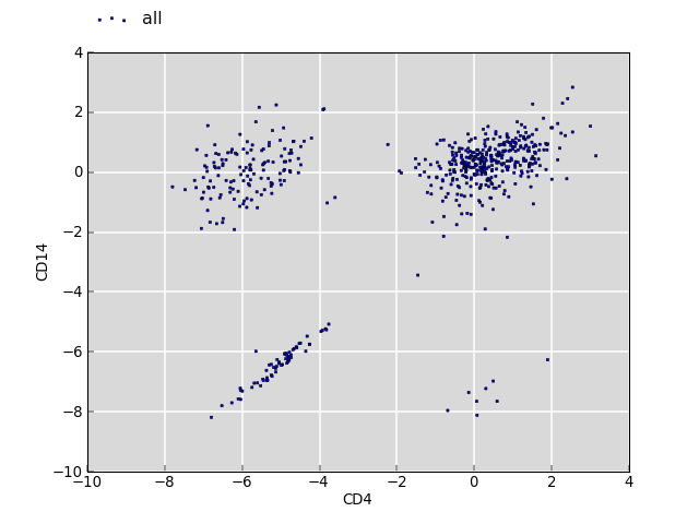
The clouds on the upper left and lower right correspond to annotations which have no overlap with CD4 but with CD14, and vice versa. The cloud around the origin of the plot shows fold changes where both overlap for CD4 and CD14 is observed. There is no bias.

The bias can be corrected by applying a constant factor that reflects the difference in the segment sizes between the two segments of interest.

Note that the pseudo-count method works well when comparing fold depletion within a single set segments of interest. Here, the intuition is that no overlap with a larger set of annotations should give higher fold depletion than if there is no overlap with a small set of annotations.

It is possible to swap the segments of interest with the annotations. However, there is a down-side. The time consuming step in gat is the randomization of the segments of interest. Thus it is benefical to test few segments of interest against many annotations. When swopped, each set in the annotations will be randomized separately and compared to a single set of segments of interest.

Note that a P-value can be prone to misinterpretation. In particular, the P-value only indicates if an observed overlap is statistically significant different from the expectation. The P-value makes no inferences about the size of the effect and if it is biologically consequential. In particular, with increasing sample size, the expectation can be measured with higher accuracy leading to smaller differences to be detectable.

Effect size

The effect size is a measure of the strength of a phenomenom. In the context of gat a useful measure of the effect size makes use of the number of segments explained by an overlap between the segments of interest and a particular annotation.

For example, an association between transcription factor binding sites and a particular annotation is likely to be more believable if it explains 20% of all transcription factor binding sites, compared to one which explains only 1% of all transcription factor binding sites. Similarly, an association that accounts for 80% of all annotations is likely to more effectual than one that accounts for only 1% of annotations.

Difference between fold changes

Gat computes assigns a statistical signficance to a fold change. The P-value, adjusted for multiple testing, reports the chance of observing the same or more extreme fold change given a neutral model. When using multiple annotations, it is thus meaningful to report the annotations for which statistically significant enrichment was found.

However, the P-value does not permit to make any inferences about the difference between two fold changes. For example, we might find that a transcription factor is 2-fold statistically enriched in promotors and 3-fold in UTRs, but we can not say with statistical confidence that the enrichment in UTRs is larger than in promotors.

Similarly, we might find that transcription factor A is 2-fold statistically enriched in promotors and transcription factor B is 3-fold enriched in promotors. Again, we can not say with statistical confidence that there is a difference in promotor binding between the two transcription factors.

The latter case, in which we have two different segments of interest and we want to contrast their fold enrichment against the same annotations is implemented in gat using the gat-compare.py command.

Briefly, the gat-compare.py command takes the observed and simulated counts from one or more gat-run.py runs. For each sample, it computes a fold change ratio as rfc = fc1 / fc2 providing a distribution of expected fold change ratios. The tool checks if the null hypothesis of no fold change difference (rfc = 1) can be rejected.

Conceptually, this works by running two simulations in-sync, one for trancription factor A and one for transcription factor B. At each iteration, the fold change is computed for each annotation between the sampled segments and the observed segments. At the same time, the fold change difference in the fold change between set A and set B is recorded. Thus, at the end of the simulations gat gets a distribution of expected fold change differences between samples and computes an empirical P-Value for the observed fold change difference between A and B.