Tutorial - Functional annnotation

This tutorial demonstrates the use of gat for functional annotation. The tutorial follows the analysis in the MacLean et al. (2010) paper introducing GREAT.

The data sets used in this tutorial are available at:

http://www.cgat.org/~andreas/documentation/gat-examples/TutorialFunctionalAnnotation.tar.gz

We are interested if the binding sites of SRF predicted from our ChIP-Seq experiment are enriched in the regulatory domains of genes of specific functions.

The data is in srf.hg19.bed. This bed formatted file contains 556 high confidence peaks from the analysis of Valouev et al. (2008) mapped to human chromosome hg19.

Functional annotation with GREAT

gat comes with a tool called gat-great that computes enrichment statistics using the binomial test implemented in GREAT.

To do an analysis as implemented in GREAT, we have prepared a bed formatted file (regulatory_domains.bed) with regulatory domains using GREAT’s basal+extension rule.

In GREAT’s definition, the regulatory domain of a gene contains a basal region and an optional extension. The basal region is defined as the region 5kb upstream and 1kb downstream of the transcription start site of a representative transcript. The basal region is then extended up to 1Mb in either direction but only up to the basal region of the closest domains.

In this example, we have used the transcription start sites of the ENSEMBL human protein coding gene set of Ensembl (release 67).

Each gene was replaced with GO terms associated with the gene obtained from the GO Gene Ontology definitions. GO terms were mapped via uniprot identifiers to genes and ancestral ontology terms were inferred.

GREAT excludes assembly gaps in the genome from the analysis. The bed formatted contigs_ungapped.bed contains all genomic regions exclusive of assembyl gaps.

We have now all data in place to run a GREAT analysis:

gat-great.py --verbose=5 \
             --log=great.log \
             --segments=srf.hg19.bed \
             --annotations=regulatory_domains.bed \
             --workspace=contigs_ungapped.bed \
             --ignore-segment-tracks \
             --qvalue-method=BH \
             --descriptions=go2description.tsv \
>& great.tsv

We also added a file go2description.tsv that contains a table with descriptions for GO identifiers.

We inserted the table into an SQL database for easy analysis. These are the top 10 results:

annotation	pvalue	observed	expected	description
GO:0015629	1.84357379006e-11	52	18.0074449104	“actin cytoskeleton”
GO:0032796	4.22734641877e-09	5	0.0557976925372	“uropod organization”
GO:0070688	1.05832288791e-07	7	0.358045266782	“MLL5-L complex”
GO:0043229	2.56771180099e-07	424	369.125027893	“intracellular organelle”
GO:0044424	3.38999777659e-07	457	406.64284565	“intracellular part”
GO:0043226	3.77332356747e-07	424	369.977837368	organelle
GO:0072303	1.28008163954e-06	3	0.0198635059219	“positive regulation of glomerular metanephric mesangial cell proliferation”
GO:0001725	1.96123184157e-06	12	2.08962341062	“stress fiber”
GO:0005634	2.30813240931e-06	295	240.687702571	nucleus
GO:0045214	2.78146278125e-06	11	1.79113154372	“sarcomere organization”

Validation against GREAT

We can check if the results are comparable to the GREAT server. We submitted our segments to GREAT, downloaded all the results into srf.great.all.tsv and loaded them into an SQL database. These are the top 10 results:

ID	BinomP	ObsRegions	ExpRegions	Desc
GO:0015629	3.064707e-11	51	17.68622	“actin cytoskeleton”
GO:0032796	4.223825e-09	5	0.05578831	“uropod organization”
GO:0045214	1.057722e-08	10	0.7800466	“sarcomere organization”
GO:0030863	2.205659e-08	16	2.666392	“cortical cytoskeleton”
GO:0001725	1.786459e-07	13	1.991518	“stress fiber”
GO:0044424	2.007378e-07	479	431.1647	“intracellular part”
GO:0070688	2.151319e-07	7	0.3981916	“MLL5-L complex”
GO:0005634	2.556219e-07	311	251.391	nucleus
GO:0032432	2.931657e-07	13	2.081847	“actin filament bundle”
GO:0043229	3.557439e-07	443	390.9065	“intracellular organelle”

The top 10 results are comparable. The same holds generally for fold change values:

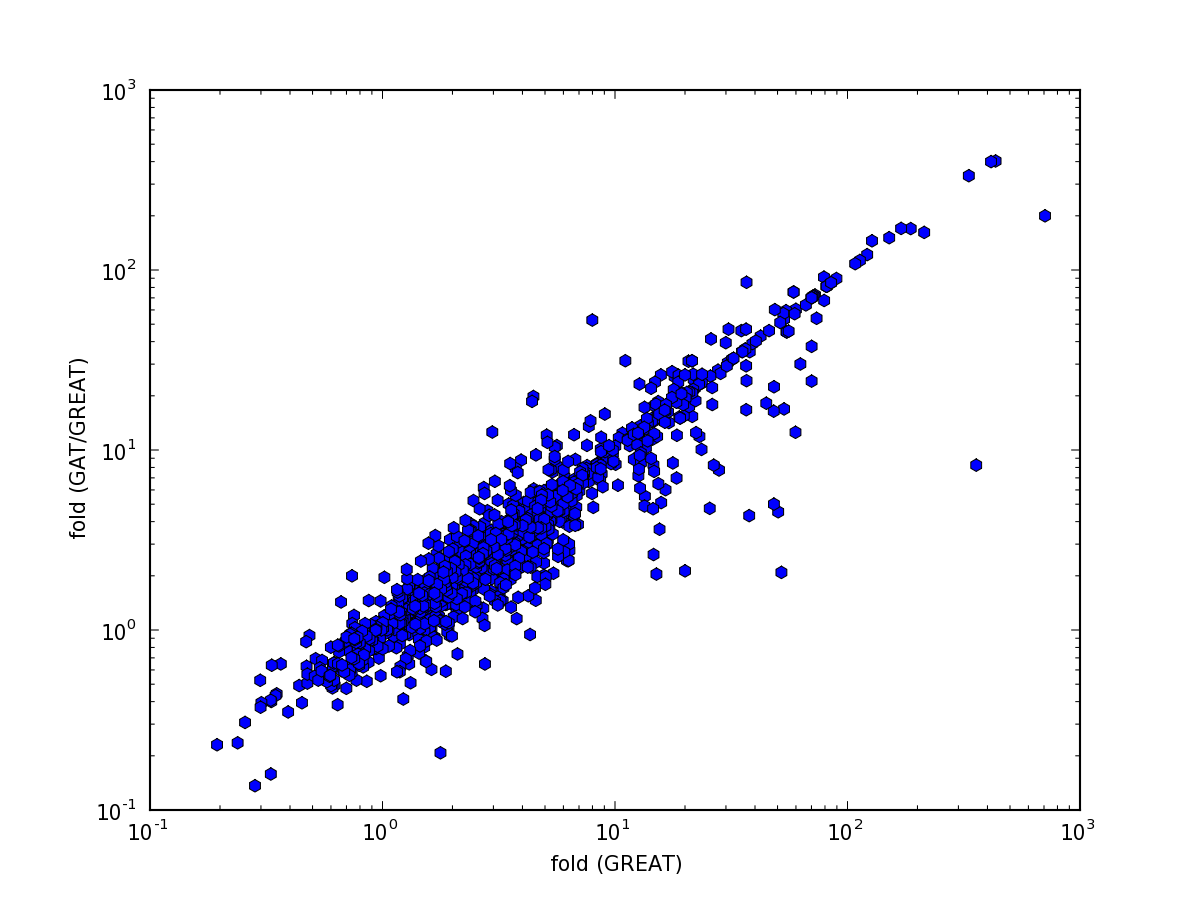
and pvalues:

Some differences are to be expected:

1. We use the ENSEMBL gene set, while GREAT uses Refseq.
2. We use a different definition of representative transcripts.
3. Our coordinates of alignment gaps might differ.
4. The assignment of GO terms to genes differ.
5. The implementations might differ in some details.

Functional annotation with gat

Gat can be run with the same input as we used for great:

gat-run.py --verbose=5 \
           --log=gatnormed.tsv.log \
            --segments=srf.hg19.bed \
            --annotations=regulatory_domains.bed \
            --workspace=contigs_ungapped.bed \
            --ignore-segment-tracks \
            --qvalue-method=BH \
            --descriptions=go2description.tsv \
            --pvalue-method=norm \
            >& gatnormed.tsv

Fold changes are very similar:

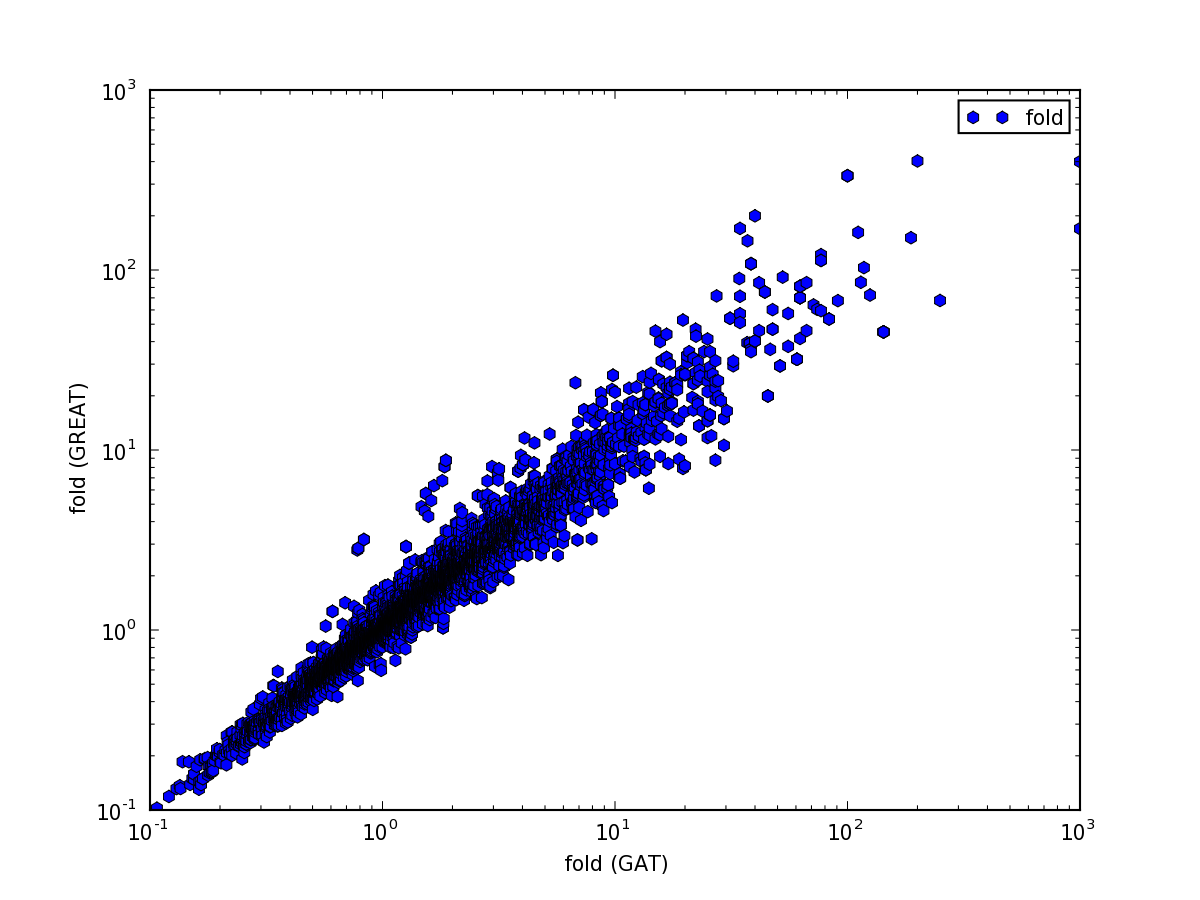
but the p-value comparison shows interesting pattern:

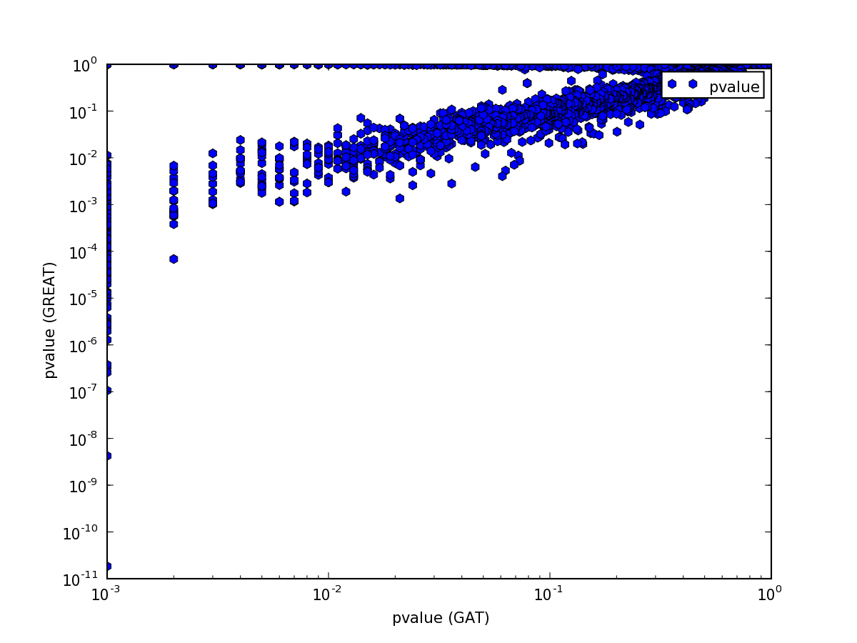
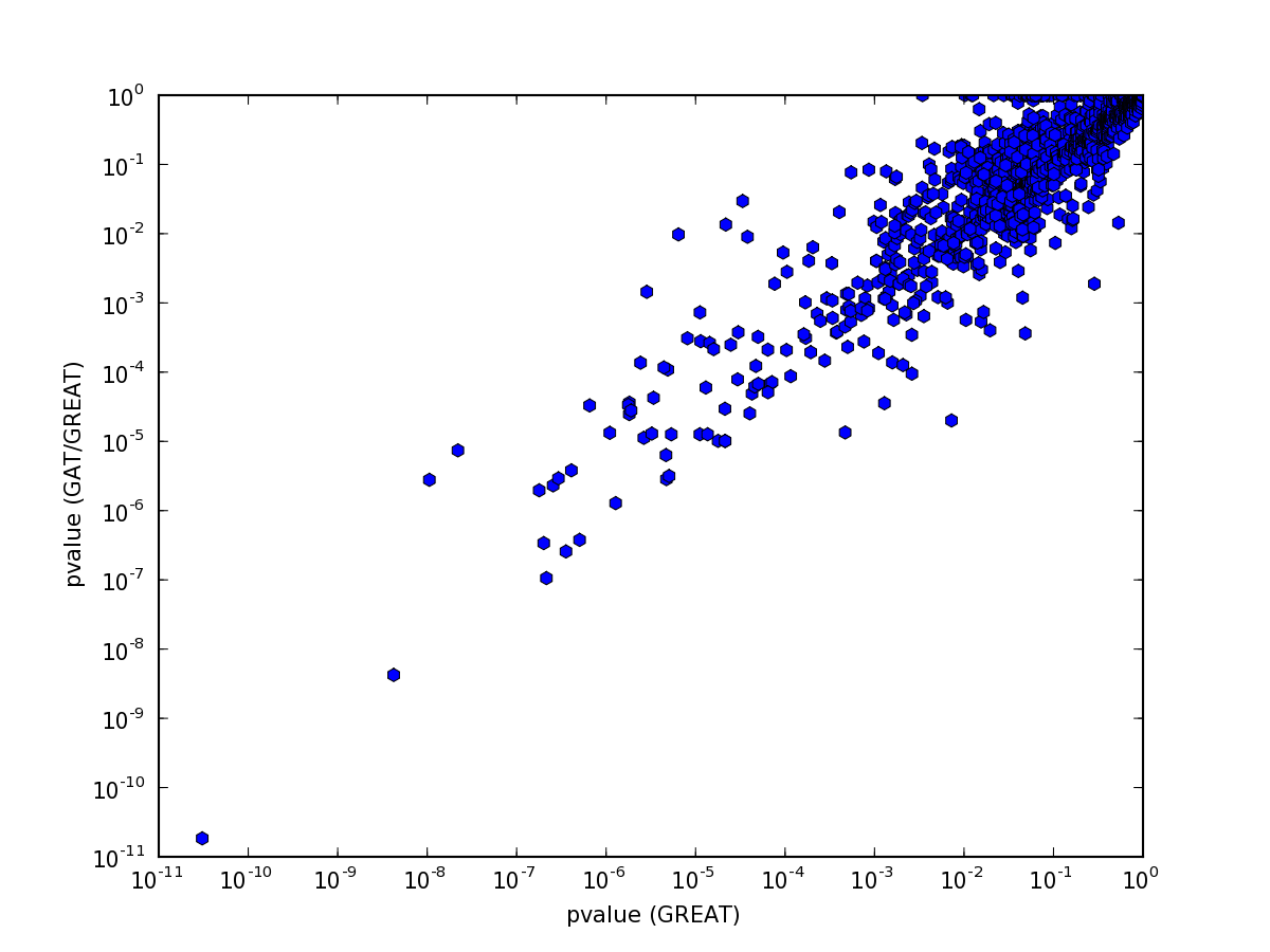
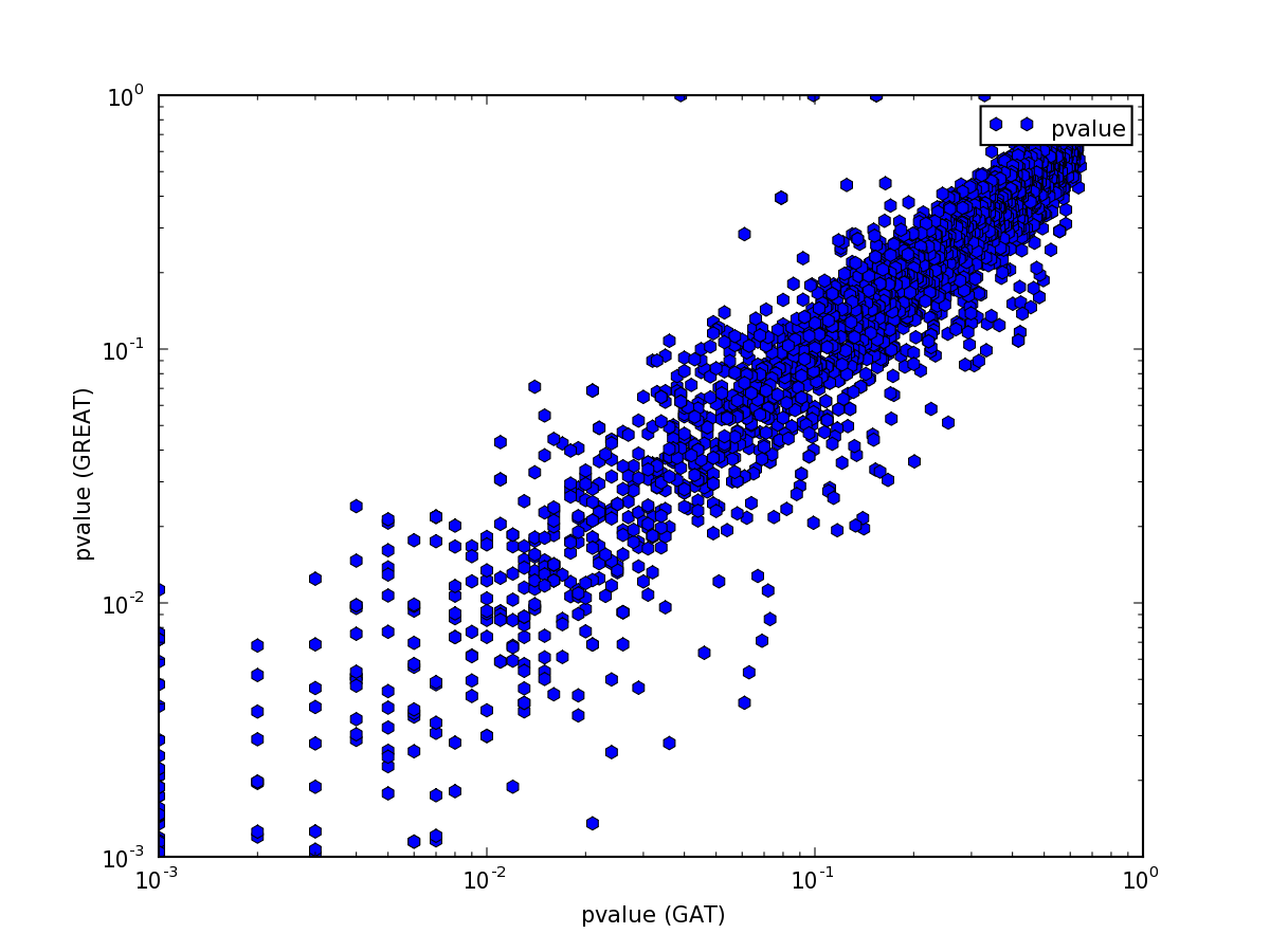
The pattern is explained easily. GREAT computes only the P-Value for enrichment, while GAT computes P-Value both for enrichment and depletion. Indeed, if we only plot p-values for annotations that are enriched, the values are comparable:

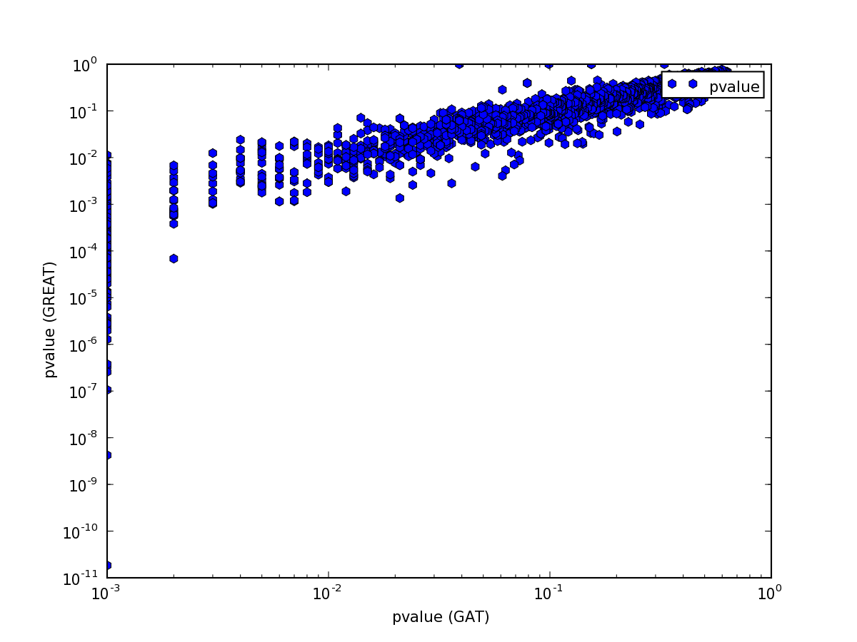
Note how the p-values are very well correlated above 10E-3:

Below a p-Value of 10E-3 the correlation breaks down. Unfortunately, the lowest empirical p-value is determined by the number of simulations performed. Adding more simulations will allow us to estimate lower p-values, but will also increase the runtime. A short-cut is to extrapolate from lower p-values by adding the option --pvalue-method=norm:

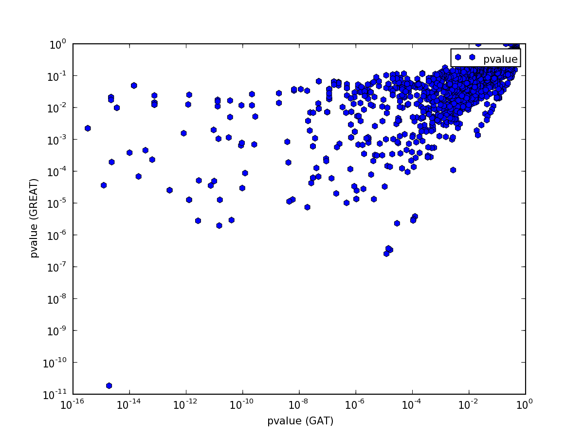
The table with enriched categories is dominated by small categories with very little expected overlap leading to very large fold changes:

annotation	pvalue	observed	expected	fold	description
GO:0043495	0.0	200	10.8	18.5185	“protein anchor”
GO:0070688	0.0	350	16.7	20.9581	“MLL5-L complex”
GO:0000212	0.0	200	9.25	21.6216	“meiotic spindle organization”
GO:0045896	0.0	150	4.65	32.2581	“regulation of transcription during mitosis”
GO:0045897	0.0	150	4.65	32.2581	“positive regulation of transcription during mitosis”
GO:0046022	0.0	150	4.65	32.2581	“positive regulation of transcription from RNA polymerase II promoter during mitosis”
GO:0046021	0.0	150	4.65	32.2581	“regulation of transcription from RNA polymerase II promoter, mitotic”
GO:0071895	0.0	100	2.7	37.037	“odontoblast differentiation”
GO:0032796	0.0	250	6.65	37.594	“uropod organization”
GO:0021593	0.0	100	2.65	37.7358	“rhombomere morphogenesis”

For interpretation of the results it is often advisable to remove annotations that are rare.

annotation	pvalue	observed	expected	fold	description
GO:0015629	3.3307e-16	2600	932.458	2.7883	“actin cytoskeleton”
GO:0044425	5.5445e-11	9620	13468.369	0.7143	“membrane part”
GO:0016021	5.7537e-11	7870	11699.204	0.6727	“integral to membrane”
GO:0031224	1.2393e-10	8220	11999.454	0.685	“intrinsic to membrane”
GO:0016020	5.5517e-08	12970	16059.768	0.8076	membrane
GO:0004888	1.0775e-06	1000	2534.458	0.3946	“transmembrane signaling receptor activity”
GO:0030029	1.1332e-06	2450	1278.537	1.9163	“actin filament-based process”
GO:0030036	1.3077e-06	2300	1174.087	1.959	“actin cytoskeleton organization”
GO:0003779	3.2187e-06	1900	963.501	1.972	“actin binding”
GO:0005886	5.2155e-06	7720	10170.117	0.7591	“plasma membrane”

Currently, we estimate fold enrichment for categories within a workspace that excludes ungapped regions. As before (Tutorial - Interval overlap), a thorough analysis should also exclude regions of low mapability.